The poison scales provide color maps inspired by the diverse colors
of Neotropical poison frogs. For discrete data it uses
ggplot2::discrete_scale(), and for continuous data it builds a smooth
gradient with ggplot2::scale_color_gradientn().
Arguments
- name
Character. Name of the poison frog palette to use one of
poison_palette_names().- type
Either
"discrete"or"continuous". Selects which kind of ggplot2 scale is constructed.- direction
Integer.
1for the palette in its stored order,-1to reverse it.- alpha
Optional numeric in
[0, 1]. Applies a uniform transparency to all colors (both discrete and continuous modes).- ...
Additional arguments passed to the underlying ggplot2 scale.
Details
Discrete: relies on an internal function factory
poison_pal()that returnsncolors (max. n = 5) on demand forggplot2::discrete_scale().Continuous: generates a 256-color gradient via
poison_palette()(type"continuous") and passes it toggplot2::scale_color_gradientn().
See also
poison_palette(), poison_pal()
Examples
require(ggplot2)
#> Loading required package: ggplot2
require(gapminder)
#> Loading required package: gapminder
require(ggridges)
#> Loading required package: ggridges
require(tibble)
#> Loading required package: tibble
require(scales)
#> Loading required package: scales
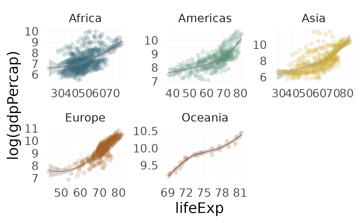
# Using `scale_color_poison()` with discrete scale
ggplot(gapminder, aes(x = lifeExp, y = log(gdpPercap), colour = continent)) +
geom_point(alpha = 0.2) +
scale_color_poison(name = "Ramazonica", type = "discrete") +
stat_smooth() +
facet_wrap(. ~ continent, scales = "free") +
theme_minimal(21, base_line_size = 0.2) +
theme(
legend.position = "none",
strip.background = element_blank(),
strip.placement = "outside"
)
#> `geom_smooth()` using method = 'loess' and formula = 'y ~ x'
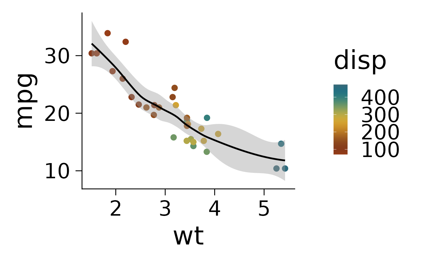
 # Using `scale_color_poison()` with continuous scale
ggplot(mtcars, aes(wt, mpg, colour = disp)) +
geom_point(size = 3) +
scale_color_poison("Ramazonica", type = "continuous", direction = -1) +
stat_smooth(col = "black") +
theme_classic(base_size = 32, base_line_size = 0.5)
#> `geom_smooth()` using method = 'loess' and formula = 'y ~ x'
# Using `scale_color_poison()` with continuous scale
ggplot(mtcars, aes(wt, mpg, colour = disp)) +
geom_point(size = 3) +
scale_color_poison("Ramazonica", type = "continuous", direction = -1) +
stat_smooth(col = "black") +
theme_classic(base_size = 32, base_line_size = 0.5)
#> `geom_smooth()` using method = 'loess' and formula = 'y ~ x'
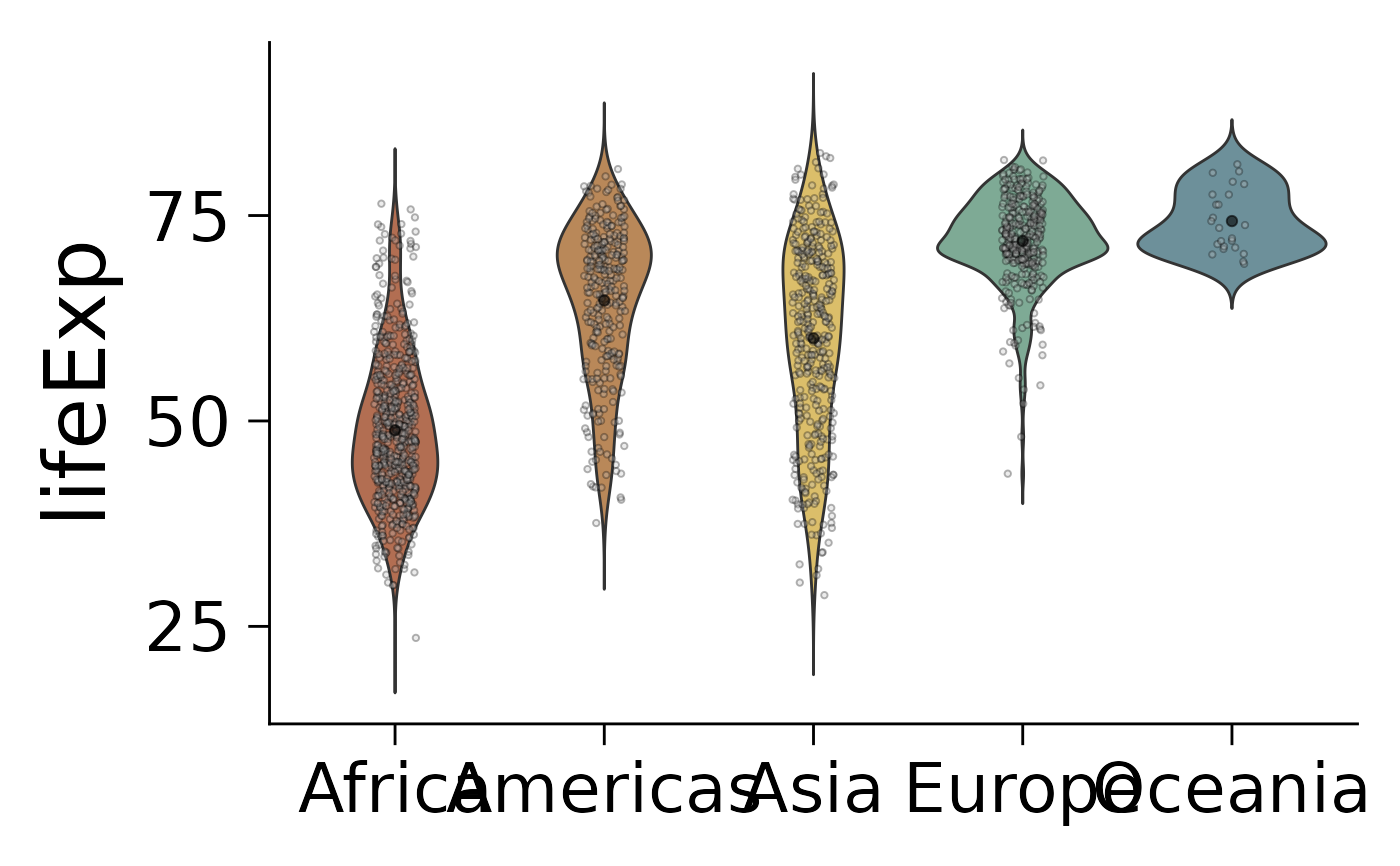
 # Using `scale_fill_poison()` with discrete scale
ggplot(gapminder, aes(x = continent, y = lifeExp, fill = continent)) +
geom_violin(trim = FALSE, alpha = 0.75) +
geom_jitter(
shape = 21,
position = position_jitter(0.1),
alpha = 0.3,
size = 0.8,
bg = "grey"
) +
stat_summary(
fun = mean,
geom = "point",
size = 1.5,
color = "black",
alpha = 0.6
) +
theme_classic(base_size = 32, base_line_size = 0.5) +
scale_fill_poison(
name = "Ramazonica",
type = "discrete",
alpha = 0.95,
direction = -1
) +
theme(legend.position = "none") +
xlab(NULL)
# Using `scale_fill_poison()` with discrete scale
ggplot(gapminder, aes(x = continent, y = lifeExp, fill = continent)) +
geom_violin(trim = FALSE, alpha = 0.75) +
geom_jitter(
shape = 21,
position = position_jitter(0.1),
alpha = 0.3,
size = 0.8,
bg = "grey"
) +
stat_summary(
fun = mean,
geom = "point",
size = 1.5,
color = "black",
alpha = 0.6
) +
theme_classic(base_size = 32, base_line_size = 0.5) +
scale_fill_poison(
name = "Ramazonica",
type = "discrete",
alpha = 0.95,
direction = -1
) +
theme(legend.position = "none") +
xlab(NULL)
 df_nottem <- tibble(year = floor(time(nottem)),
month = factor(month.abb[cycle(nottem)],
levels = month.abb),
temp = as.numeric(nottem))
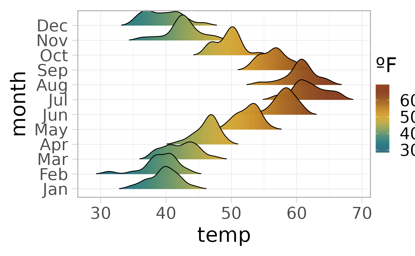
# Using `scale_fill_poison()` with continuous scale
ggplot(df_nottem, aes(x = temp, y = month, fill = stat(x))) +
geom_density_ridges_gradient(scale = 2, rel_min_height = 0.01) +
scale_fill_poison(
name = "Ramazonica",
type = "continuous",
alpha = 0.95,
direction = 1
) +
labs(
fill = "ºF") +
theme_light(base_size = 26, base_line_size = 0.5) +
theme(
legend.position = "right",
legend.justification = "left",
legend.margin = margin(0,0,0,0),
legend.box.margin = margin(-20,-20,-20,-20)
)
#> Warning: `stat(x)` was deprecated in ggplot2 3.4.0.
#> ℹ Please use `after_stat(x)` instead.
#> Picking joint bandwidth of 0.942
df_nottem <- tibble(year = floor(time(nottem)),
month = factor(month.abb[cycle(nottem)],
levels = month.abb),
temp = as.numeric(nottem))
# Using `scale_fill_poison()` with continuous scale
ggplot(df_nottem, aes(x = temp, y = month, fill = stat(x))) +
geom_density_ridges_gradient(scale = 2, rel_min_height = 0.01) +
scale_fill_poison(
name = "Ramazonica",
type = "continuous",
alpha = 0.95,
direction = 1
) +
labs(
fill = "ºF") +
theme_light(base_size = 26, base_line_size = 0.5) +
theme(
legend.position = "right",
legend.justification = "left",
legend.margin = margin(0,0,0,0),
legend.box.margin = margin(-20,-20,-20,-20)
)
#> Warning: `stat(x)` was deprecated in ggplot2 3.4.0.
#> ℹ Please use `after_stat(x)` instead.
#> Picking joint bandwidth of 0.942