pTRAPPING

pTRAPPING takes the raw count data from a TRAP-seq or PhosphoTRAP experiment and finds which genes are specifically enriched in your cell population of interest — all in a few lines of R. You give it a counts table where every sample column is labelled with its treatment group, replicate number, and whether it is IP (immunoprecipitated) or INPUT (total RNA); the package figures out the rest. Three functions cover the full workflow: differential expression with your choice of statistical engine (ptrap_de()), a classic volcano plot for one condition (ptrap_volcano()), and a paired scatter plot to compare two conditions head-to-head (ptrap_volcano2()).

Installation

# install.packages("devtools")
devtools::install_github("laurenoconnelllab/pTRAPPING")

Dependencies from Bioconductor (edgeR, limma, DESeq2) are installed automatically.

Functions at a glance

Function	What it does
ptrap_de()	Differential expression: IP vs INPUT. Six statistical methods.
ptrap_volcano()	Volcano plot for a single condition.
ptrap_volcano2()	Scatter plot comparing two conditions side-by-side.

Quick start

Get differential expression results of interesting genes from your counts matrix in just a few lines of code:

library(pTRAPPING)

# Load counts matrix
counts.mat <- read.delim(
  system.file("extdata", "TAN_etal_2016_raw.txt", package = "pTRAPPING")
)

# Table of differentially expressed genes of interest for one condition using the default method "LRT" from edgeR
ptrap_de(
  counts_mat = counts.mat,
  treatment_name = "PACAP",
  kable.out = TRUE,
  genes.filter = c(
    "Adcyap1",
    "Bdnf",
    "Ucn3",
    "Gng8",
    "Fosl2",
    "Junb",
    "Trappc12",
    "Gfap"
  )
)

Gene	logFC	logCPM	LR	PValue	FDR	treatment	diffexpressed
Gng8	4.056	5.578	39.952	<0.001	<0.001	PACAP	UP
Ucn3	3.949	5.218	25.454	<0.001	<0.001	PACAP	UP
Bdnf	4.338	3.090	23.035	<0.001	<0.001	PACAP	UP
Trappc12	-3.345	1.809	10.679	0.001	0.030	PACAP	DOWN
Gfap	-2.979	5.086	10.628	0.001	0.031	PACAP	DOWN
Fosl2	0.781	6.990	3.694	0.055	0.304	PACAP	NO
Adcyap1	1.516	3.665	2.708	0.100	0.398	PACAP	NO
Junb	0.757	4.568	1.385	0.239	0.600	PACAP	NO

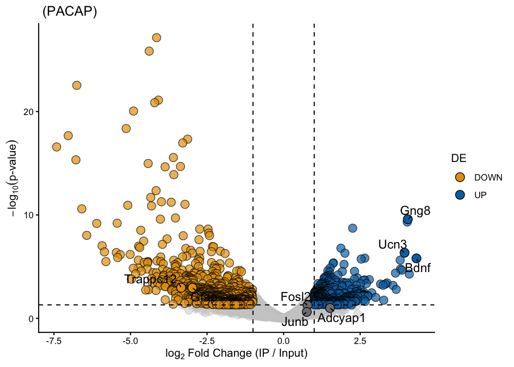
Plot the same results in a volcano plot and annotate any genes of interest:

# Volcano plot — label a few genes of interest
ptrap_de(
  counts_mat = counts.mat,
  treatment_name = "PACAP"
) |>
  ptrap_volcano(
    fdr = FALSE, # use raw p-values (n=3; FDR is very conservative)
    genes.annot = c(
      "Adcyap1",
      "Bdnf",
      "Ucn3",
      "Gng8",
      "Fosl2",
      "Junb",
      "Trappc12",
      "Gfap"
    )
  )

Check Getting started with pTRAPPING to see how to run the full workflow, including comparing two conditions head-to-head and making interactive volcano plots!

References

• The PhosphoTRAP method was introduced in:

Knight, Z.A., Tan, K., Birsoy, K., Schmidt, S., Garrison, J.L., Wysocki, R.W., Emiliano, A., Ekstrand, M.I., and Friedman, J.M. (2012). Molecular profiling of activated neurons by phosphorylated ribosome capture. Cell 151, 1126–1137. https://doi.org/10.1016/j.cell.2012.10.039

• Bioconductor packages used for differential expression analysis:

edgeR: Robinson, M.D., McCarthy, D.J., and Smyth, G.K. (2010). edgeR: a Bioconductor package for differential expression analysis of digital gene expression data. Bioinformatics 26, 139–140. https://doi.org/10.1093/bioinformatics/btp616

limma: Ritchie, M.E., Phipson, B., Wu, D., Hu, Y., Law, C.W., Shi, W., and Smyth, G.K. (2015). limma powers differential expression analyses for RNA-sequencing and microarray studies. Nucleic Acids Res 43, e47. https://doi.org/10.1093/nar/gkv007

DESeq2: Love, M.I., Huber, W., and Anders, S. (2014). Moderated estimation of fold change and dispersion for RNA-seq data with DESeq2. Genome Biol 15, 550. https://doi.org/10.1186/s13059-014-0550-8

• The example dataset is from:

Tan, C.L., Cooke, E.K., Leib, D.E., Lin, Y.-C., Daly, G.E., Zimmerman, C.A., and Knight, Z.A. (2016). Warm-sensitive neurons that control body temperature. Cell 167, 47–59. https://doi.org/10.1016/j.cell.2016.08.028