Getting Started with pTRAPPING

What problem does pTRAPPING solve?

Imagine you want to know which genes are actively being read — translated into protein — in a specific, rare cell type buried inside a complex tissue like the brain. You cannot easily sort those cells out; they are intermingled with hundreds of other cell types. TRAP-seq and PhosphoTRAP are molecular techniques that let you tag ribosomes (the cellular machinery that reads genes) in your target cells, and then pull them out with their attached RNA. The RNA you capture in this immunoprecipitation step — the IP fraction — reflects what your target cells were actively translating. You keep the leftover, un-pulled RNA too — the INPUT fraction — as a reference for total gene expression in the tissue.

The core question is then: which genes are enriched in the IP relative to the input? A gene enriched in IP is being translated in your target population; a gene depleted in IP is present in the tissue but not in your cells of interest. Answering this question requires normalising the data, picking a statistical test, adjusting for multiple comparisons across thousands of genes, and visualising the results — all of which pTRAPPING handles for you with three functions.

PhosphoTRAP adds one more layer: instead of constitutively tagging ribosomes, it captures only ribosomes that carry a phosphorylated form of the S6 protein — a marker of recent neural activation. This means you can ask not just “which genes are translated in these cells?” but “which genes are translated in these cells right now, after a specific stimulus?”. The experimental design is otherwise identical: IP fraction (activated cells’ RNA) vs. INPUT fraction (total tissue RNA).

The example datasets: Tan et al. (2016)

Throughout this vignette we use data from Tan et al. (2016) Cell 167, 47–59, a landmark PhosphoTRAP study in mice.

Dataset 1: Identify warm-sentive neurons Experiment: To identify which genes are highly enriched in warm-sensitive neurons, mice were challenged with heat and phosphorilated ribosomes in neurons that fired in response were isolated by immunoprecipitation. RNA from immunoprecipitates was sequenced and fold-enrichment for each gene was calculated as IP/Input fractions. This data set has RPKM normalized counts (counts per million, scaled by TMM-adjusted library sizes, and divided by gene length in kilobases) for 8863 genes across 3 biological replicates (3 mice - IP and Input sample each).

library(pTRAPPING)
library(dplyr)
library(tibble)

# Pre-computed RPKM values — already normalised; use with norm.method = "none"
warm_counts <- read.delim(
  system.file("extdata", "warm_counts.txt", package = "pTRAPPING")
)

dim(warm_counts) # 8863 genes × 9 columns (1 gene-ID + 8 samples)
#> [1] 13724     7
names(warm_counts) # column names encode treatment, fraction, and replicate
#> [1] "Gene"      "WC1_INPUT" "WC1_IP"    "WC2_INPUT" "WC2_IP"    "WC3_INPUT"
#> [7] "WC3_IP"

The column names follow the convention pTRAPPING expects: each name contains a treatment label (WC - warm-cells), a fraction keyword (IP or Input), and a replicate number (1 or 2), in any order and separated by underscores. The function parses these automatically — no metadata table needed.

Step 1 — Differential expression with `ptrap_de()`

ptrap_de() compares the IP fraction to the INPUT fraction for a given treatment group and returns a ranked table of genes based on four available methods. Use this table as a quick guide to pick you model and normalisation method:

Feature	DESeq2	edgeR LRT	edgeR QLF	limma/voom
Normalization	Median-of-ratios (geometric)	TMM	TMM	Quantile normalization
Core assumption	Most genes not DE	Most genes not DE	Most genes not DE	No DE assumption; matches distributions
How it works	Per-gene ratio to geometric mean → median ratio = size factor	Weighted mean of log-ratios vs. reference; trims extreme genes	Same as LRT	Forces identical count distributions across all samples
What is scaled	Raw counts ÷ size factor	Library sizes (indirect)	Library sizes (indirect)	Full distribution remapped per sample
Statistical model	Negative binomial GLM + dispersion shrinkage	NB GLM; likelihood ratio test	NB GLM; quasi-likelihood F-test	Linear model; `voom` precision weights handle count variance
Test statistic	Wald test (default) or LRT	Chi-squared LRT	F-test with empirical Bayes squeezing	Moderated t/F-test (empirical Bayes)
Dispersion estimation	Shared + gene-wise + MAP shrinkage	Common → trended → tagwise	Common → trended → tagwise + QL dispersion	Mean-variance trend via `voom`
Small sample behavior	Good; shrinkage stabilizes estimates	Conservative; can be anti-conservative with few replicates	Better than LRT with few replicates; QL adds extra variance component	Good; empirical Bayes borrows strength across genes
Key functions	`estimateSizeFactors()`, `DESeq()`	`calcNormFactors()`, `glmFit()`, `glmLRT()`	`calcNormFactors()`, `glmQLFit()`, `glmQLFTest()`	`normalizeQuantiles()`, `voom()`, `lmFit()`
Data type	RNA-seq counts	RNA-seq counts	RNA-seq counts	Microarrays (native); RNA-seq via `voom`
Strengths	Small n; LFC shrinkage	Well-established; fast	More reliable with small n; recommended over LRT for most RNA-seq	Large datasets; microarrays; complex linear models
Bioconductor pkg	`DESeq2`	`edgeR`	`edgeR`	`limma`

All three GLM-based methods ("LRT", "QLF", "deseq") and the LM-based "voom" normalise the data internally — you do not need to normalise first. For the t-test methods you can choose a normalisation via norm.method:

`norm.method`	When to use
`"CPM"` (default)	Raw counts; comparable across replicates of the same gene
`"RPKM"`	Raw counts + gene lengths available via `gene.length`; needed for cross-gene comparisons within a sample
`"mratios"`	Raw counts; DESeq2-style size-factor normalisation
`"none"`	Data already normalised (e.g., a pre-computed RPKM matrix)

Note on "RPKM": this option requires you to supply gene lengths via gene.length (a named numeric vector, in base pairs). Without it, the function will throw an error. When you already have a pre-normalised matrix — as in the Tan et al. dataset below — use norm.method = "none" instead.

Note on filter = FALSE: by default, ptrap_de() removes low-expression genes using filterByExpr, which expects raw integer counts. When passing a pre-normalised matrix (RPKM, TPM, or similar), the small floating-point values will mislead the filter and cause real genes to be dropped. Set filter = FALSE whenever norm.method = "none" is used with a pre-normalised input.

Calculating gene fold enrichment and p-values with the paired t-test

We use the paired t-test — the same approach as the original paper. Tan et al. ran the test on RPKM values, so we pass the pre-normalised RPKM matrix and set norm.method = "none" and filter = FALSE to skip any additional normalisation step. Also, pior.count is set to 0 because RPKM values are already normalised and do not require a pseudocount.

warm_de <- warm_counts |>
  dplyr::filter(dplyr::if_any(dplyr::where(is.numeric), ~ .x > 1)) |> #keep counts > 1
  ptrap_de(
    treatment_name = "WC", # only one treatment group in this dataset
    test_method = "paired.ttest",
    norm.method = "none", # data are pre-normalised
    filter = FALSE, # skip count-based filtering
    prior.count = 0 # no pseudocount needed for RPKM values
  )

The function prints a message showing what it auto-parsed from the column names: treatments, replicate numbers (blocks), and fractions. The argument “paired.ttest” in the test_method argument (as well as “unpaired.ttest”) returns a named list including $results and $fe tables. Inspect the result:

# The paired.ttest method always returns a named list
names(warm_de)
#> [1] "results" "fe"

# $results: one row per gene, sorted by p-value
head(warm_de$results)
#> # A tibble: 6 × 7
#>   Gene     logFC t_statistic    PValue   FDR treatment diffexpressed
#>   <chr>    <dbl>       <dbl>     <dbl> <dbl> <chr>     <chr>        
#> 1 Xpr1    -0.775      -210.  0.0000226 0.178 WC        NO           
#> 2 Slain1  -1.98       -152.  0.0000435 0.178 WC        NO           
#> 3 Larp6   -0.717      -149.  0.0000453 0.178 WC        NO           
#> 4 Zfp187  -0.827      -135.  0.0000548 0.178 WC        NO           
#> 5 Gm10032 -0.617       -95.5 0.000110  0.209 WC        NO           
#> 6 Wars2   -0.735       -91.9 0.000118  0.209 WC        NO

`$results`: per-gene differential expression.

The $results output is a tibble with one row per gene, sorted by p-value. The columns include log fold change (logFC), p-value, FDR, and a classification of whether the gene is differentially expressed (DE) based on user-defined thresholds for logFC and FDR. By default, the function uses a logFC threshold of 1 (meaning a 2-fold change) and an FDR threshold of 0.05 to classify genes as “UP” (enriched in IP), “DOWN” (depleted in IP), or “NO” (not DE).

Understanding the output columns

Column	What it means
`Gene`	Gene identifier
`logFC`	log2(IP / INPUT) — positive = enriched in target cells
`PValue`	Raw p-value from the paired t-test
`FDR`	Benjamini-Hochberg adjusted p-value (false discovery rate)
`diffexpressed`	`"UP"` (enriched), `"DOWN"` (depleted), or `"NO"`

The diffexpressed column is determined by two thresholds (both must be met):

lfc_threshold — minimum absolute logFC (default 1, meaning ≥ 2× change)
fdr_threshold — maximum FDR (default 0.05)

You can change these without re-running the analysis — ptrap_volcano() and ptrap_volcano2() recompute the classification from your chosen thresholds.

`$fe`: per-animal fold enrichments

The paired t-test also returns a $fe tibble with each animal’s IP/INPUT fold enrichment (FE) for every gene. This is useful for spot-checking individual genes or running your own downstream analyses.

# Per-animal fold enrichment for the top 5 genes
head(warm_de$fe, 5)
#> # A tibble: 5 × 5
#>   Gene           FE_1  FE_2  FE_3 log2_mean_FE
#>   <chr>         <dbl> <dbl> <dbl>        <dbl>
#> 1 0610007C21Rik 0.314 0.627 1.17       -0.507 
#> 2 0610007L01Rik 0.930 0.734 0.522      -0.457 
#> 3 0610007P08Rik 0.678 0.522 0.315      -0.985 
#> 4 0610007P14Rik 0.394 0.848 1.64       -0.0572
#> 5 0610007P22Rik 1.01  1.17  1.11        0.136

Step 2 — Visualise the results with `ptrap_volcano()`

A volcano plot puts logFC on the x-axis and statistical significance (-log p-value) on the y-axis. Genes in the upper-right corner are both strongly enriched and statistically significant — the most interesting candidates. Genes in the upper-left are strongly depleted. Grey points fail one or both thresholds. If interactive = FALSE (default), labels are always shown for the genes in genes.annot (if specified).

warm_de$results |>
  ptrap_volcano(
    fdr = FALSE, # use raw p-values (n=3; FDR is very conservative)
    log_base = 2, # -log2(p) on y-axis, matching Tan et al. 2016
    point_alpha = 0.3,
    genes.annot = c(
      "Fosl2",
      "Egr2",
      "Bdnf",
      "Adcyap1",
      "Junb",
      "Fosb",
      "Rrad",
      "Gadd45b"
    ) # known warm-sensitive markers
  )

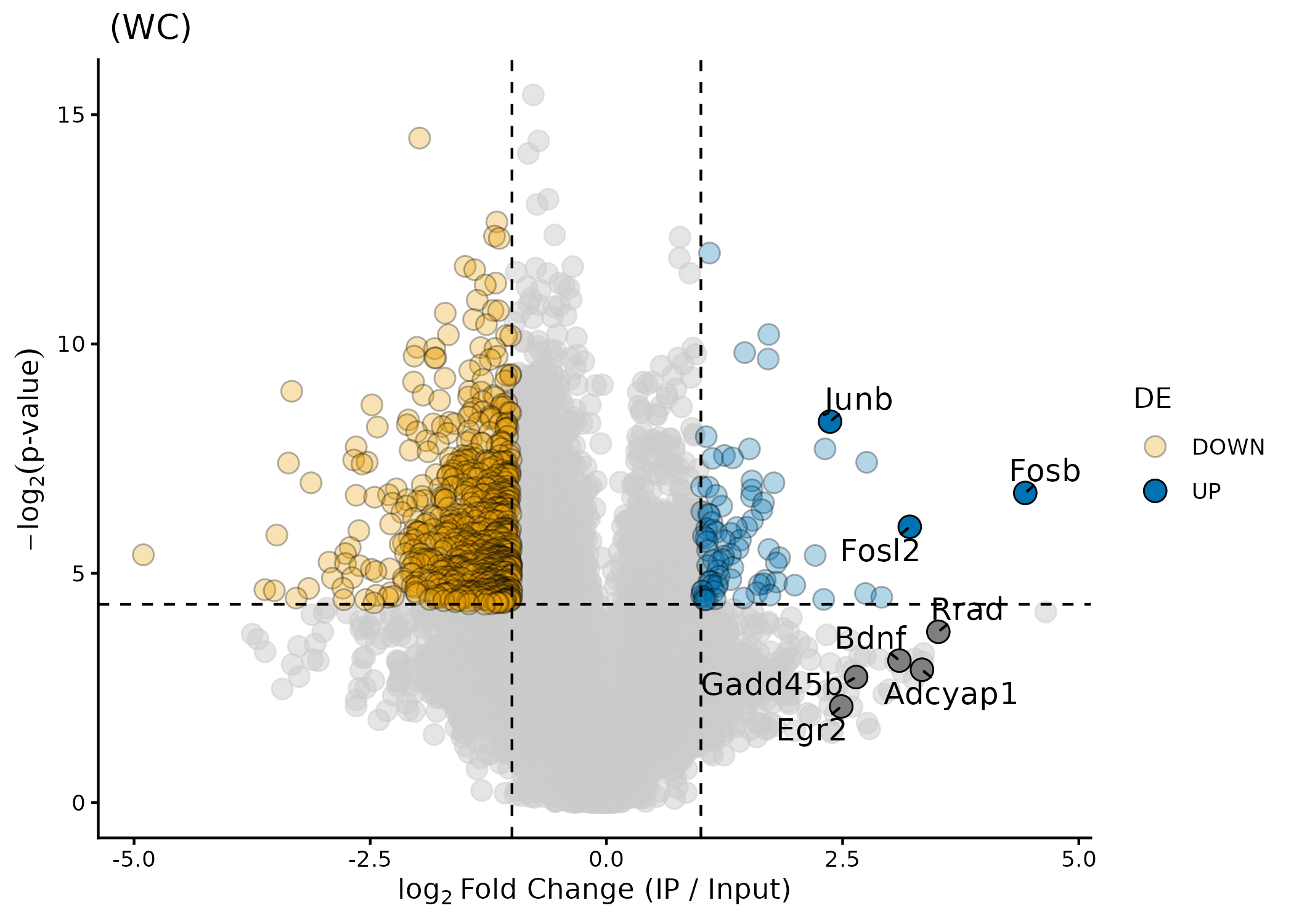
Volcano plot showing known warm-sensitive markers in Tan et al. (2016).

When interactive = TRUE, the plot becomes interactive via Plotly and users can zoom in and hover over points to see gene labels, logFC, p-value, and FDR.

warm_de$results |>
  ptrap_volcano(
    fdr = FALSE,
    log_base = 2, # -log2(p) on y-axis, matching Tan et al. 2016
    point_alpha = 0.3,
    interactive = TRUE) # hover to show gene labels and info

Volcano plot showing known warm-sensitive markers in Tan et al. (2016).

Key arguments:

Argument	Default	What it does
`fdr`	`TRUE`	Use FDR (`TRUE`) or raw p-value (`FALSE`) for the y-axis and colouring
`lfc_threshold`	`1`	logFC cutoff for the vertical dashed lines
`fdr_threshold`	`0.05`	p-value cutoff for the horizontal dashed line
`log_base`	`10`	Base of the log transform on the y-axis
`genes.annot`	`NULL`	Character vector of gene names to label
`title`	auto	Plot title (defaults to region + treatment)

Customising colours

Pass a named vector to override the defaults:

warm_de$results |>
  ptrap_volcano(
    fdr = FALSE,
    colors = c("UP" = "#D55E00", "DOWN" = "#56B4E9"),
    title = "Volcano plot — custom colours"
  )

The function returns a ggplot2 object, so you can add or override any layer with standard ggplot2 syntax:

library(ggplot2)

warm_de$results |>
  ptrap_volcano(fdr = FALSE) +
  theme(plot.title = element_text(face = "bold")) +
  xlim(-10, 10)

Step 3 — Compare two conditions with `ptrap_volcano2()`

Dataset 2: Characterising warm-sensitive neurons Experiment: The authors created BDNF-Cre and PACAP-Cre transgenic mice and used TRAP to sequence the genes expressed in these warm-sensitive neuron populations. This data set has RPKM normalized counts for 8863 genes across 2 biological replicates (2 mice - IP and Input sample each) for both BDNF-Cre and PACAP-Cre lines.

# Pre-computed RPKM values — already normalised; use with norm.method = "none"
counts_rpkm <- read.delim(
  system.file("extdata", "TAN_etal_2016_RPKM.txt", package = "pTRAPPING")
)

dim(counts_rpkm) # 8863 genes × 9 columns (1 gene-ID + 8 samples)
#> [1] 8863    9
names(counts_rpkm) # column names encode treatment, fraction, and replicate
#> [1] "Gene"          "PACAP_Input_1" "PACAP_IP_1"    "PACAP_Input_2"
#> [5] "PACAP_IP_2"    "BDNF_Input_1"  "BDNF_IP_1"     "BDNF_Input_2" 
#> [9] "BDNF_IP_2"

Run ptrap_de() for both conditions separately to get two DE result tables, which are the input for ptrap_volcano2().

pacap_de <- counts_rpkm |>
  filter(dplyr::if_any(dplyr::where(is.numeric), ~ .x > 1)) |> #keep counts > 1
  mutate(gene = make.unique(Gene)) |>
  column_to_rownames("gene") |>
  #round() |>
  ptrap_de(
    test_method = "paired.ttest",
    norm.method = "none",
    treatment_name = "PACAP",
    filter = FALSE,
    lfc_threshold = 0.3,
    prior.count = 0
  )

# Inspect the per-gene fold enrichment
pacap_de$fe
#> # A tibble: 8,863 × 4
#>    Gene       FE_1  FE_2 log2_mean_FE
#>    <chr>     <dbl> <dbl>        <dbl>
#>  1 Adcyap1    7.87  6.64         2.86
#>  2 Bdnf       4.98 10.1          2.91
#>  3 Ucn3       6.80 30.4          4.22
#>  4 Gng8       8.47 18.6          3.76
#>  5 Nme4       5.26 15.3          3.36
#>  6 Nxph4     11.0  20.6          3.98
#>  7 Hist1h2bg 13.5   1.72         2.93
#>  8 Ghrh       4.41  9.91         2.84
#>  9 Hist1h4m   5.54  4.82         2.37
#> 10 Samd3      5.44  6.43         2.57
#> # ℹ 8,853 more rows

bdnf_de <- counts_rpkm |>
  filter(dplyr::if_any(dplyr::where(is.numeric), ~ .x > 1)) |> #keep counts > 1
  mutate(gene = make.unique(Gene)) |>
  column_to_rownames("gene") |>
  #round() |>
  ptrap_de(
    test_method = "paired.ttest",
    norm.method = "none",
    treatment_name = "BDNF",
    filter = FALSE,
    lfc_threshold = 0.3,
    prior.count = 0
  )

# Inspect the per-gene fold enrichment
bdnf_de$fe
#> # A tibble: 8,863 × 4
#>    Gene        FE_1   FE_2 log2_mean_FE
#>    <chr>      <dbl>  <dbl>        <dbl>
#>  1 Adcyap1    6.16   9.05          2.93
#>  2 Bdnf       2.77   5.30          2.01
#>  3 Ucn3      14.3    7.96          3.47
#>  4 Gng8       7.38  12.7           3.33
#>  5 Nme4       9.51   4.21          2.78
#>  6 Nxph4      3.35   4.66          2.00
#>  7 Hist1h2bg  0.400 14.2           2.87
#>  8 Ghrh       6.31   5.17          2.52
#>  9 Hist1h4m  15.2    0.455         2.97
#> 10 Samd3      4.85   7.39          2.61
#> # ℹ 8,853 more rows

BDNF and PACAP cells co-express both BDNF and PACAP genes and almost the same set of genes, including Unc3, Nxph4, Ghrh, etc.

Then ptrap_volcano2() places both results on a single 2D scatter plot:

x-axis: logFC for condition 2
y-axis: logFC for condition 1
Diagonal (dotted): genes enriched equally in both
Above diagonal: more enriched in condition 1
Below diagonal: more enriched in condition 2

Genes that meet the significance thresholds in both conditions, in only one, or in neither are shown in distinct colours.

ptrap_volcano2(
  de_result_1 = pacap_de$results,
  de_result_2 = bdnf_de$results,
  fdr = FALSE,
  interactive = TRUE
)

Scatter comparison of PACAP and BDNF enrichment. Genes on the diagonal are enriched equally in both conditions.

Genes near the diagonal are similarly enriched in both PACAP and BDNF cells.

Customising colours

The three DE classes are named after the treatment labels in your data. Pass a colors vector using those names:

ptrap_volcano2(
  pacap_de$results,
  bdnf_de$results,
  fdr = FALSE,
  colors = c(
    "DE in both" = "#D55E00",
    "DE only PACAP" = "#0072B2",
    "DE only BDNF" = "#009E73"
  )
)

Common issues

“Cannot identify IP/INPUT fraction in column name”: The parser could not find an IP or INPUT keyword. Check your column names and use ip_level / input_level to match your exact spelling (e.g., input_level = "Input" for mixed case).
“Cannot identify a replicate number in column name”: Every sample column must contain a digit for the replicate number (e.g., 1, 2, 10). Add a number to your column names or supply sample_df manually.
FDR column is all NA or very few significant genes: With n = 2, multiple-testing correction is extremely conservative. Try fdr = FALSE in the volcano functions. With ≥ 4 replicates and a GLM method, FDR-based calls are more reliable.
norm.method = "RPKM" requires gene.length: Gene lengths (in base pairs) must be provided as a named numeric vector whose names match the gene IDs in your count matrix. These are available from annotation packages such as TxDb.* or via BioMart. If you already have a pre-normalised RPKM matrix, use norm.method = "none" instead — no lengths needed.

What problem does pTRAPPING solve?

The example datasets: Tan et al. (2016)

Step 1 — Differential expression with ptrap_de()

Calculating gene fold enrichment and p-values with the paired t-test

$results: per-gene differential expression.

Understanding the output columns

$fe: per-animal fold enrichments

Step 2 — Visualise the results with ptrap_volcano()

Customising colours

Step 3 — Compare two conditions with ptrap_volcano2()

Customising colours

Common issues

Step 1 — Differential expression with `ptrap_de()`

`$results`: per-gene differential expression.

`$fe`: per-animal fold enrichments

Step 2 — Visualise the results with `ptrap_volcano()`

Step 3 — Compare two conditions with `ptrap_volcano2()`